Post-Modern Portfolio Theory And The Sortino Ratio

In a prior post I performed a cursory analysis of modern portfolio theory (MPT) and showed that some of the theory's assumptions were violated in the real world. However, this should come as no surprise. MPT's inventor, Harry Markowitz, knew of the short comings but chose them out of praticality. At the time, asset price data was limited and computers were not able to process vast amounts of data or compute the results of complex algorithms like they are today. So, Markowitz defined assumptions that enabled tractable analytical and computational solutions to his theory.

Since the development of MPT, some progress has been made in relaxing the Gaussian assumptions that constrain asset return distributions. This progress has been captured in what is known as Post-Modern Portfolio Theory (PMPT), which was conceived in the early 1990's. There are other frameworks that take different but related approaches to portfolio construction, such as the Fama-French Three Factor Model.

Sortino Ratio

The Sortino Ratio is a modified version of the Sharpe Ratio. The Sharpe Ratio, which is defined as, \[ S_a = \frac{E[R_a - R_f]}{\sigma_a}, \] measures a portfolio's performance by taking the ratio of excess return to volatility, or standard deviation of excess return. A high positive Sharpe Ratio indicates an asset yields high positive returns and a low volatility. A low Sharpe Ratio means the asset's excess returns are small relative to its volatility. For all the reasons we mentioned in the prior post, this can be a flawed measure. Beyond that, the measure does not distinguish between positive and negative volatility, treating them both the same. But in reality, investors may place different values on positive and negative variation in returns.

This is where the Sortino Ratio comes into play. The ratio $S$ is computed as \[ S = \frac{R - T}{dr}, \] where $R$ is the assets annual rate of return, $T$ is an investor's target return, and $dr$ is the asset's downside risk. The denominator $dr$ is defined as \[ dr = \sqrt{\int_{-\infty}^T (T-r)^2 f(r) dr} \] where $f(r)$ is a probabilty distribution intended to reflect the likelihood of the asset producing a return of $r$. The structural properties of $f(r)$ are not part of the metric, meaning skewed distributions with heavy tails can be selected to capture rates of return that could be produced by the asset, observed or not. This is an important difference that we will discuss more below.

Another difference between $S$ and $S_a$ is $T$. The Sortino Ratio does not require the use of a risk free rate. Instead, it allows an investor to select a target rate of return. In addition to this flexibility, $dr$ contains two characteristics that make $S$ more robust than its predecessor. The first is its ability to only account for downside risk. The second is weighting the downside risk probabilistically via $f(r)$. These traits are captured holistically by integrating over the domain that is less than or equal to the target return $T$.

This structure provides a flexible framework for incorporating investor objectives and weighting asset return characteristics that work against achieving specified goals probabilistically. Moreover, they can be made to reflect real-world dynamics better than a traditional Gaussian approach due to incorporation of $f(r)$.

Calculating the Sortino Ratio

The procedure to compute the Sortino Ratio for a portfolio is straightforward. The first step requires computing annualized returns for the portfolio or asset. In the code snippet and analysis below, we used data from the VTI ETF provided by Yahoo! finance. Next, an appropriate probability distribtion representing return characteristics of the asset must be selected. After selecting the distribution, it should be fit to the data using an appropriate method, like maximum likelihood.

The next phase of the procedure computes $dr$. As shown in the code snippet, this can be done using a numerical integration routine like the one provided in scipy. Once $dr$ is calculated, computing $S$ is trivial. We simply take the difference between the mean annual return and target return and divide it by $dr$.

      
        import csv
        import numpy as np
        from scipy.stats import lognorm
        from scipy.integrate import quad
        
        # roughly annualize the returns using data from yahoo finance
        vti = [i for i in csv.reader(open('VTI.csv'))][1:]
        vti = [float(i[-2]) for i in vti]
        annualized_returns = [(vti[i*365] - vti[365*(i-1)]) / vti[(i-1)*365] 
                              for i in range(1,14)]

        # fit data to a lognormal using MLE
        s, loc, scale = lognorm.fit(annualized_returns)
        rv = lognorm(s, loc, scale)
        
        # compute sortino ratio
        R = np.mean(annualized_returns)
        T = 0.1
        result, err = quad(lambda i: (T-i)**2 * rv.pdf(i), -np.inf, T)
        dr = np.sqrt(result)
        sortino_ratio = (R - T) / dr
      
      

Analyzing Behavior

Now that we have an understanding of the metric and how to compute it, we can (briefly) study its behavior, using historical stock market data and two heavy tailed probability distributions.

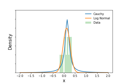
The figure below plots annual return data from the VTI ETF beteen June 15, 2001 and November 27, 2020 along with the estimated Lognormal and Cauchy distributions. Both were fit using maximum likelihood methods. The mean annual return of VTI, $R$, over this period was approximately 11.7%. It is worth noting that the Lognormal distribution produces lower tail probabilities than the Cauchy.

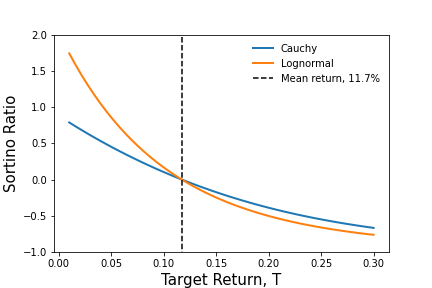
Using the data and the distributions, we then compute $S$ over a range of $T$ values ($T \in (0,0.3)$) to gain an sense for how $S$ varies with return targets and distribution choice. The figure below shows how $S$ changes with $T$. The figure shows two regimes, one where $T$ is greater than $R$, denoted by the black dashed line, and the other where it less.

For $T > R$, the value of $S$ is roughly the same, regardless of distribution choice. This is due to the fact that both distributions have similar values in this range.

For $T < R$, the value of $S$ diverges between the Cauchy and Lognormal distributions. Looking back at the first figure, it is not difficult to understand what is going on. As we mentioned earlier, the Cauchy has more density than the Lognormal in the range below $R$. As a result, the value of $f(r)$ in this regime will be larger, thus making $dr$ larger and $S$ smaller.

This structure suggests that $S$ is sensitive, as it should be, to the choice of distribution, to the extent that they differ in certain regimes of interest, mainly, the regime where $T \le R$.

Conclusions

While the Sortino Ratio has properties that make it more flexible to probabilistically quantify performance of assets relative to a user specified target return, it still relies on a taking a mean value, which can be misleading with dealing with heavy tailed structure. Moreover it relies on historical data to make assumptions and forecasts about the future. That being said, its generalization of the Sharpe Ratio make it a viable alternative for investors wanting to emphasize returns falling below their desired target.