Measures Of Entropy For Time Series
Entropy
Entropy is a concept used to describe the disorder or uncertainty of a system. Since it's conception in thermodynamics, it has found use cases across many other areas of science, both phyical and theoretical. Perhaps one of the most important applications was in the domain of information theory. Even more recently, entropy has found its way into the fields of neuroscience and finance.
The field of neuroscience has developed a comprehensive theory that unifies our biological and theoretical understanding of the brain's function, explaining how and why it has evolved the way it has over time. This theory is known as the free-energy princple and says that the brain is running a bayesian optimization algorithm to minimize the rate at which it is surprised by its environment, subject to a dynamic heirarchy of needs, such as hunger and thirst. By doing so, the brain minimizes the amount of energy it expends learning how to respond to its environment, thus trending towards a state of homeostasis and ultimately maximizing its ability to survive expending the least amount of work.
The free-energy principle is a useful and natural way to think about decisions and risk. In essence, portfolio theory can be re-cast as a free energy minimization concept, where investors are continuously trying to maximize their returns, and thus their chances of survival by avoiding surprise, which is equivalent to avoiding losses. Recasting the problem in this way enables the use of entropy as part of the traditional investment risk-reward framework without the reliance on assumptions such as finite variance that lead to systematic underestimation (see a prior post on modern portfolio theory) of risk and as a result lower chances of survival and lower returns.
With this as background and motivation, the rest of this blog post reviews a select number of entropy measures and then applies those measures to both synthetic and empirical data number of securities. In a future post, we will incorporate these measures into modern portfolio theory and compare it to the traditional approach of using variance.
Measures of Entropy
Shannon Entropy
Shannon entropy, typically denoted as \( H(X) \), quantifies the uncertainty of a system, \( X \), using the following equation: $$H(X) = -\sum_{i=1}^n p(x_i)\log p(x_i),$$ where \( p(x_i) \) is the probability of observing value \( x_i \). Note that this expression of entropy is discrete and requires one to know the probability values. The sum of these probabilities multiplied \( \log \) returns the total number of bits needed to encode information contained in the distribution. Intuitively, as uncertainty increases, so does the number of bits needed to encode it. Similarly, as uncertainty decrease, the number of bits needed to encode the information decreases. In the field of telecommunications, this relationship is used to determine how many bits are needed to encode a message, send it across a noisy channel, and recover it at the receiver.
In the case of flipping an unbiased coin, \( H(X) = -\frac{1}{2} \log(\frac{1}{2}) - \frac{1}{2} \log(\frac{1}{2}) = 1 \), requires a single bit to encode the state it is in. This makes sense, the coin be in either heads or tails state with equal probability and to represent two states using a single bit, we need two symbols, 0 and 1.
What if the coin was biased and being in a heads state had a probability of 0.8 and tails 0.2? The entropy would then be \( H(X) = -0.8 \log(0.8) - 0.2 \log(0.2) = 0.722 \), which is less than 1 in the prior example. this makes sense since it is much more likely that the coin will be in a heads state than tails and as the relationship states, lower uncertainty corresponds to lower entropy.
Approximate Entropy
Like many others, financial systems are typically studied as function of time. Moreover, financial time series are typically correlated over varying periods, both long and short. And finally, in many cases we don't know, or want to assume, all the values the times series could assume. As a result, a measure of entropy that analyzes fluctuations through time without strict boundaries can be considered superior to one that analyzes parametric or bounded probability distributions. Approximate entropy addresses these concerns.
Approximate entropy attempts to measure the amount of uncertainty in a time series by analyzing the regularity of the series using a simple algorithm that requires two parameters: \( m, r\). \( m \) is used by the algorithm to break up a time series into smaller windows of size \( m \) and \( r \) is used as a filtering threshold when two windows are compared with each other.
Specifically, a time series is broken up into a series of windows of size \( m \). For each pair of windows, their distance is computed as \( d(x_a, x_b) = \max_{i} |x_a(i) - x_b(i)| \). Using these windows, the fraction of windows with a distance less than or equal to \( r \) when compared to \( x_i \) is calculated. Mathematically, this is expressed as: $$ C(i,m,r) = \frac{ \sum_{j=1}^{N-m}\Bbb{I} [d(x_i, x_j) \le r]}{N - m + 1}. $$
Approximate entropy is then computed as: $$ ApEn = \phi^m(r) - \phi^{m+1}(r) $$ where $$ \phi^m(r) = \frac{\sum_{i=1}^{N-m+1} \ln C(i,m,r)}{N-m+1} $$ Like other measures of entropy, ApEn takes on small values when a time series is repetitive and large values when it is not.
Sample Entropy
Sample entropy is a modification of ApEn to address some of its limitations, including measuring self-similarity. Using a similar approach as ApEn, a time series is broken up into windows of size \( m \) (These are also referred to as templates). Then, the distance between templates is computed using \( d(x_a, x_b) = \max_{i} |x_a(i) - x_b(i)| \), just like ApEn. Finally, SampEn is computed by taking the negative natural log of sum of the template pairs of length \( m \) with distance less than \( r \) divided by the sum of the template pairs of length \( m + 1 \) with distance less than \( r \). Mathematically, this is expressed as $$ SampEn = -\log \frac{\sum_{i=1}^{N-m+1} \sum_{j=1}^{N-m} \Bbb{I} [d(x_i, x_j) \le r]} {\sum_{i=1}^{N-m+2} \sum_{j=1}^{N-m+1} \Bbb{I} [d(x_i, x_j) \le r]}. $$
Permutation Entropy
Permutation entropy is another measure of uncertainty for time series. As in the prior examples, entropy is computed by first breaking a time series into windows, also referred to as embeddings in this method, of size \( n \). Next, each embedding is compared to the permutation set to determine which permutation it matches. The total counts for each permutation are recorded and turned into probabilities by dividing each count by the total number of embeddings. Using these probabilities entropy is then computed using the traditional Shannon entropy equation: $$ H(X) = -\sum_{i=1}^n p(x_i) \log p(x_i) $$
As an example, consider a time series of \( s(t) = 10,5,1,3 \) and an embedding value of 2. When \( n=2 \), there 2 embedding permutations: one where \(s(t) < s(t+1) \) and one where \(s(t) > s(t+1) \). Comparing each embedding to these permutations and counting up their occurenances leads to 1 count of \(s(t) < s(t+1) \) and 2 counts of \(s(t) > s(t+1) \) and a total of 3 embeddings. Using these values, we compute the permutation entropy as: $$ H(X) = -\frac{1}{3}\log\frac{1}{3} - \frac{2}{3}\log\frac{2}{3} = 0.637$$
Summary of Methods
We have reviewed four measures of entropy. Each was created for a specific purpose, with the last three designed to describe the uncertainty of systems expressed as time series. In the table below we highlight each measure, the basic formula, and the strenghts and limitations of the method, including the complexity of the algorithm used to compute the measure.
| Entropy | Formula | Parameters | Strengths | Limitations |
|---|---|---|---|---|
| Shannon | \( H(X) = -\sum_{i=1}^{n} p(x_i)\log p(x_i) \) |
|
|
|
| Approximate | \( ApEn = \phi^m(r) - \phi^{m+1}(r) \) | \( m, r \) |
|
|
| Sample | \( SampEn = -\log \frac{\sum_{i=1}^{N-m+1} \sum_{j=1}^{N-m} \Bbb{I} [d(x_i, x_j) \le r]} {\sum_{i=1}^{N-m+2} \sum_{j=1}^{N-m+1} \Bbb{I} [d(x_i, x_j) \le r]} \) | \( m, r \) |
|
|
| Permutation | \( H(X) = -\sum_{i=1}^{n} p(x_i)\log p(x_i) \) | \( n, \tau \) |
|
|
Now we briefly analyze the methods perform using two simple time series, one that is
structured and periodic and the other that is random. The time series are plotted below.
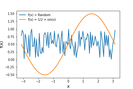
Using intuition we have described above, we should expect the orange time series to have a lower entropy than the random time series for each and every measure of entropy described thus far. The table below shows the results and confirms this hypothesis.
| Entropy measure | \( f(x) = Random(\{0 \dots 1\}) \) | \( f(x) = \frac{1}{2} + \sin(x) \) |
|---|---|---|
| Shannon | 6.64 | 5.34 |
| Approximate | 1.00 | 0.129 |
| Sample | 1.617 | 0.128 |
| Permutation | 0.984 | 0.442 |
Conclusion
This post reviewed the concept of entropy and showed how various measures, specifically derived for systems that produce times series signals, consistently quantify system disorder. This finding and entropy's occurence in human nature, specifically its use in the free-energy principle of the brain, motivates its use within the world of finance, where cash flows, share prices, and many signals are expressed as time series and decisions are often made to maximize returns while simultaneously avoiding surprise.
In a future post, we will incorporate entropy into portfolio construction and performance analysis to test the hypothesis that using entropy as a measure of risk leads to at least identical returns but with lower risk when compared to modern portfolio theory and its reliance on variance.