Safe Leads In Basketball
With the playoffs in full swing, I thought some analysis of the scoring dynamics in basketball would interest readers, so I've put together a comparison of two methods for predicting a game's winner - one developed by a serious sports fan and the other developed by myself, in collaboration with Aaron Clauset.
In 2008, Bill James published a formula for determining when a lead is safe in a basketball game, which I'm calling the Safe Lead method. Bill's calculation is as follows:
- Take the number of points one team is ahead and subtract 3.
- Add 1/2 a point if the team that is ahead has the ball, and subtract a 1/2 point if the other team has the ball. (Numbers less than zero become zero.)
- Square the result.
- If the squared result is greater than the number of seconds remaining in the game, the lead is safe.
Why does this formula work? And perhaps more importantly, how accurate is it? In this post, I'll shed some light on the accuracy of Bill's formula, and I'll also compare it to a method I've developed, which is based upon viewing a basketball game as a stochastic process.
At this point, readers that are only interested in the results might want to scroll to the end of this post.
Data
For this analysis, a data set that describes when baskets were scored, and by which team, during a game, is required. Both the NBA and ESPN have made available, high resolution, play-by-play data of nearly every basketball game played in recent history. I've written a Python script to download and extract play-by-play data from ESPN, which can be found here.
I'm using data from the last 10 seasons of the NBA. In total, this is roughly 12,000 games and 1,200,000 scoring events (I'll define what a scoring event is shortly). For my analysis, I'm using a Python library I've created called SportsSciPy.
Basketball as a stochastic process
When the game of basketball is viewed as though it were a stochastic process, we can model the probability of the home team's score increasing by \(p\) points as the joint probability of observing a scoring event, the home team winning the event, and the event being worth \(p\) points. Mathematically, this can be expressed as \[\begin{aligned} \Pr(\Delta S_{home} = p) = \Pr(\textrm{event})(t)\Pr(\textrm{home team scores})\Pr(\textrm{points = }p). \end{aligned} \] I've used a similar model in previous research on modeling scoring dynamics in online games. In what follows, I'll analyze the data non-parametrically with respect to each of the three components introduced above: timing, scoring, and points. A paper that performs a more rigorous and parametric analysis of what I'll be presenting below can be found here.
Timing
To get started, we'll begin by studying the timing of scoring events. A scoring event is defined as the total number of points scored during a second of official game play. This means a series of foul shots scored in the same second of play are aggregated into a single event worth a point value equal to the number of successful shots made by the player. The figure below plots the probabilty of observing a scoring event at each second of a game.
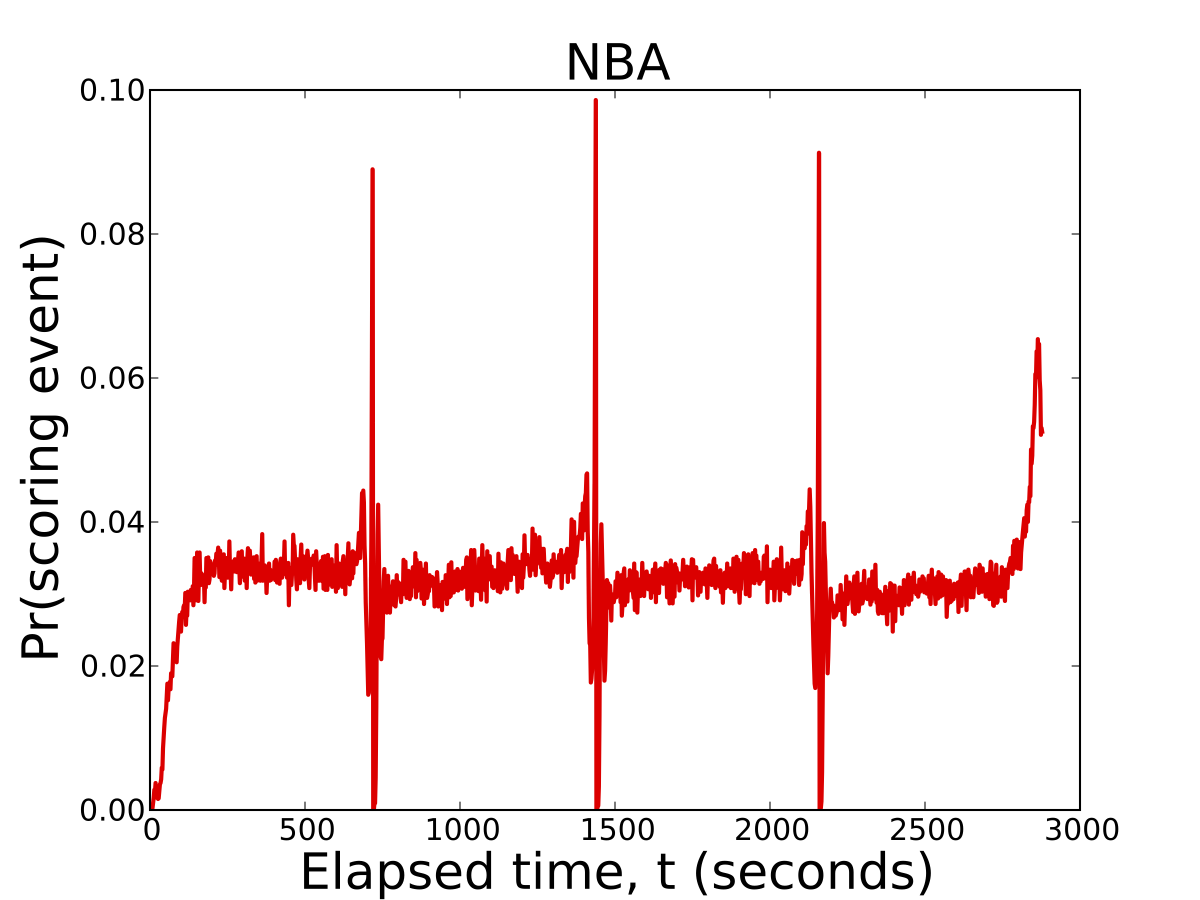
To fans, this figure should agree well with their intuition and understanding of the game. The 4 spikes in scoring at seconds 720, 1,440, 2,160, and 2,880 are the last seconds of play in each quarter of the game. In the first quarter, the probability of scoring is nearly constant once teams warm up and find their rhythm. Scoring in the second quarter steadily increases going into half-time. In the second half, scoring occurs with relatively constant probability, with the exception of roughly the last 30 seconds of the game, where teams pick up tempo to try and secure their win or reduce their deficit.
The figure and inset below plot the distribution of inter-arrival times between consecutive scoring events as well as their correlation. They tell us about two important features of the game. First, there is roughly a 30 second delay between consecutive baskets and second, that events are virutally uncorrelated.
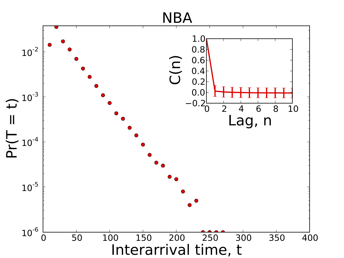
These features suggest the timing of scoring events are independent, thus making it possible to estimate the number of scoring events remaining in a competition as follows
\[\begin{aligned} \textrm{Number of remaining scoring events, }n = \sum_{t=i}^{2880} \Pr(\textrm{event})(t). \end{aligned} \]Scoring
Next, we'll examine how the probability of scoring correlates with a team's lead size. The figure below plots the probability of scoring given a lead size of \(l\) points.
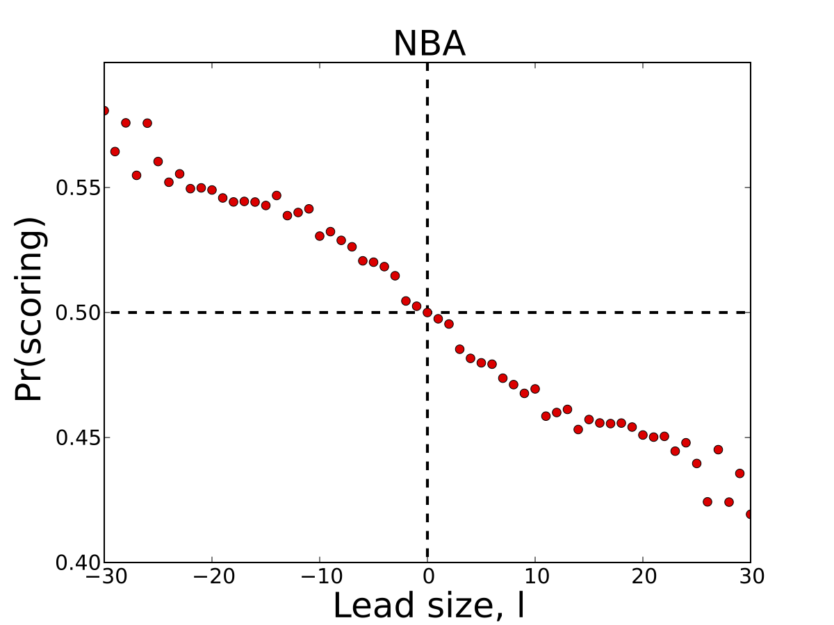
Perhaps one of the most interesting features of basketball is that the probability of scoring again decreases as a team's lead increases. Some have spectulated that this negative correlation is due to the possesion change after each successful event. However, I have found that in other sports with the same rule, such as football, the probability of scoring increases with lead. If you have an opinion or some insight that may explain this phenonmenon, please share in the comments of this post.
Points
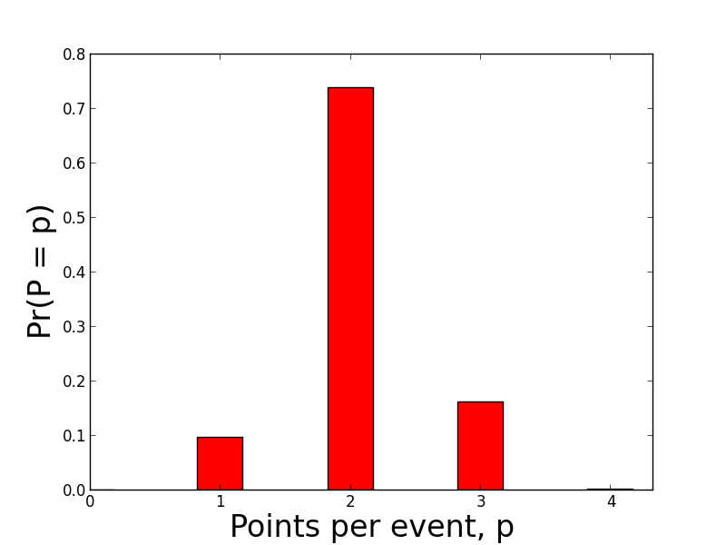
Finally, we'll briefly examine the distribution of points scored over all the games in our data set. As expected, the majority of scoring events are worth 2 points.
Predicting a game's outcome
Now that we have identified the data and methods for estimating each component of our scoring dynamics model, we can create a Markov chain that describes the evolution of a game's lead. For consistency, we'll let a game's lead, \(l\), be \(> 0\) when the home team is in the lead and \(l\) be \( < 0\) when the away team is in the lead.
The Markov chain's state space consists of score differences between the home and away team. The transition probabilities are equal to the joint probability of scoring given the lead size and the value of scoring event. These values can be stored in a matrix, denoted as \(P\), where \(P_{ij}\) is equal to the probability of transitioning from a current lead of \(i\) to future lead of \(j\). Mathematically the probability of transitioning from state \(i\) to state \(j\) is equal to
\[\begin{aligned} P_{ij} = \Pr(\textrm{scoring }| \textrm{ lead}) \Pr(\textrm{points} = p). \end{aligned} \]Given \(P\), all that is required to compute the probability of one team winning, given the game's current state, is to estimate the number of remaining events in the game, \(n\), raise \(P\) to this power, and then sum over all states that are either greater or less than 0 (depending on team). Mathematically this is equal to
\[\begin{aligned} \Pr(\textrm{home team wins } | \textrm{ }l,n) = \sum_{j=1}^k P^n_{lj}. \end{aligned} \]Performance
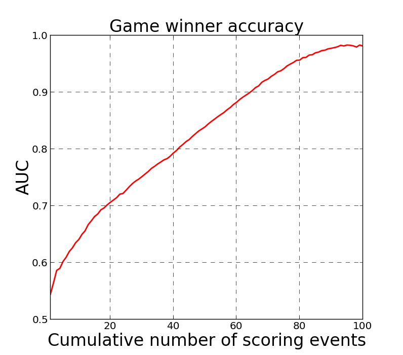
To measure the performance of the Markov chain's ability to predict a game's outcome, I've computed the timing, scoring, and points distributions using 3/4 of the game data and then predicted each remaining game's outcome as a function of cumulative number of scoring events. The figure below plots the model's prediction performance, using AUC, which can be interpretted as the accuracy of the classifier, as a function of cumulative events. If we assume a scoring event every 30 seconds, then the classifier operates at roughly 75% accuracy after 15 only minutes of play, and continues to improve as the game progresses.
Comparison to Bill James' Safe Lead Method
So how does our Markov chain method of estimating a game's winner compare to Bill James' Safe Lead method? First, let's take a closer look at what Bill's method is telling us.
The Safe Lead method predicts whether or not the current leader of a game will lose their lead. This means that if Bill's method predicts a safe lead, the team in the lead will win the game. On the other hand, if Bill's method predicts the lead isn't safe, it does not mean that the team in the lead will lose the game. Rather, it tells us that the opposing team is likely to take over the lead at some point later in the game. This means we can't directly compare the prediction method shown above with the Safe Lead method.
To do a proper comparison using our Markov model, we need to calculate a slightly different estimate - the probability that the leading team changes at least once in the remaining \(n\) scoring events of the game. Mathematically, this is equivalent to the probability of the lead, \(l\), ending in a state \(j\), where \( 0 < j \le m\) if \( l < 0 \) or \( -m \le j < 0\) if \( l > 0 \), summed over the remaining steps in the game, \(n\). For example, if \(l < 0 \), then the probability of the leader changing at least once is equal to
\[\begin{aligned} \Pr(\textrm{leader changes} | \textrm{ }l,n) = \frac{1}{n}\sum_{i=1}^n \sum_{j=1}^m P^i_{lj}. \end{aligned} \]The figure below plots the AUC of each method as a function of time in the last quarter of the game. I've left off the first 3/4 of game time because the Safe Lead method doesn't do any better than chance.
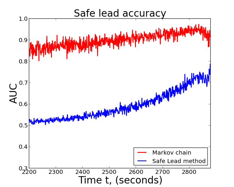
From the results above, it's clear that the Markov chain classifier drastically outperforms Bill's method. However, this isn't to say the Safe Lead method is bad or incorrect. The main reason Safe Lead operates at a lower accuracy rate than the Markov chain is because it's more conservative. That is to say, when the Safe Lead method predicts a lead is safe, it's almost always right, but when it predicts a lead isn't safe, it's often times incorrect. If you're familiar with confusion matrices, this means the Safe Lead method has a high true positive rate and a high false negative rate.
Conclusions
In this post, I've presented a probablistic model of scoring dynamics in basketball and used it to construct a Markov chain that can make predictions about observing different types of scoring events in a game. I've also analyzed Bill James' Safe Lead method, presented a comparison to a Markov chain method, and showed that it has higher accuracy than the Safe Lead method.
For fans who like to watch streaming statistics of scoring events, I've created a web application, onthespotsports.com, that provides real time predictions for a variety of scoring events including the ones reviewed here. The site is viewed best on up-to-date versions of Chrome, Firefox, and Safari.